 北大中文核心期刊

Scheduling theory is an important sub-area in Operations Research, where the operations to be executed are generally referred to as jobs and the facilities execute the operations are referred to as machines. Besides the inter-relationships between the jobs and the machines that describe how the jobs should be processed by the machines, there are intra-relationships among the machines and intra-relationships among the jobs. One class of job intra-relationships is the precedence, which specifies the constraints that some jobs have to be finished before some other jobs can be started. Numerous industrial applications lead to various precedence constrained scheduling problems[1], which have received much algorithmic study since their emergence.
Graham[2] proposed the precedence constrained multiprocessor scheduling to minimize the makespan, or
If the processing time of a job on every machine is one unit, that is,
Table 1 Complexity and approximability results on precedence constrained scheduling
| Problem | Complexity | Approximation | |
| NP-hard[2] | |||
| NP-hard to | |||
| NP-hard | |||
| NP-hard open[9] | |||
| PTAS open[10] | |||
| Not APX-hard[11] | |||
| Strongly NP-hard[13, 14] | |||
| Strongly NP-hard[13, 14] | |||
| NP-hard open | |||
| P[16, 17] | |||
| P[15, 16] | |||
| Strongly NP-hard[14, 18] | |||
| NP-hard open | |||
| P[15, 16] | |||
The machines in the multiprocessor scheduling are identical and a job needs to be processed by only one of them. In an open-shop or a flow-shop of
Given a precedence graph, by noting that the precedence relation is transitive, we may remove the "redundant" precedence constraints from the graph, and thus we may assume without loss of generality that there are no redundant constraints in the given precedence graph. Then, a constraint in the precedence graph specifies a job is the immediate predecessor of the other job (or the other way around, the latter job is the immediate successor of the former). If each job has at most one immediate successor (predecessor, respectively), then the precedence graph is an intree (outtree, respectively). Bräsel et al.[17] proved that
In this paper, we study the two problems
In the next section we introduce definitions and the preprocessing of the precedence graph to partition the jobs into layers, and construct the so-called spine of the graph[19]. In Section 3 we deal with open-shop scheduling, present a maximum matching scheme between the singletons, which are on the spine, and the jobs outside of the spine, and show that the resulting approximation algorithm has the same performance ratio of
1 Definitions and Preliminaries
We use
If
If neither
The following preprocessing of the precedence graph to partition the jobs into agreeable layers is presented in [19]. Given the precedence graph
One sees that a longest (directed, omitted in the sequel) path in the precedence graph
Using the layered representation
Theorem 1The layered representation
Let
If
2 A matching-based approximation for $ O \mid prec, p_{ij} = 1 \mid C_{\max} $
Consider an instance of
In the sequel, the first number in the subscript of a job/vertex refers to the level of the job/vertex. For example,
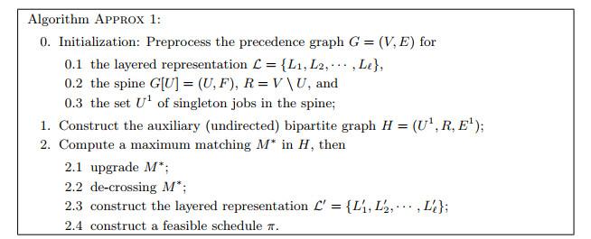
In the first step of the approximation algorithm Approx 1 (of which a high-level description of the algorithm Approx 1 is depicted in Fig. 2), an auxiliary (undirected) bipartite graph
Fig.1
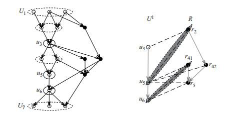
Fig.1
A precedence graph
Fig.2
The following lemma summarizes some structural properties of the bipartite graph
Lemma 1In
Proof The proof is done by contradiction and the transitivity of the precedence relation.
Note that the singleton job
For the example illustrated in Figure 1, where
Given a matching in the bipartite graph
Lemma 2In
Proof Let
Note that for each singleton job
Given a matching in the bipartite graph
Lemma 3In
Proof Given a matching
When there are two crossing edges
From
Lemma 4A non-upgradeable and non-crossing matching
Proof Let
One sees that each
Next we want to prove that if
When
When both
Let
This finishes the proof of the lemma. We remark that from the given matching
The above analysis motivates the following second step of the algorithm Approx 1, in which a maximum (cardinality) matching
We have showed the makespan of the schedule achieved by the algorithm Approx 1 in Eq. (2). For the approximation ratio, we will prove next an improved lower bound on the minimum makespan using the number
Consider an optimal schedule
Assume the unit time interval
Afterwards, no more edge incident at
Lemma 5Given an optimal schedule
Proof In the constructed edge subset
If a singleton job
This finishes the proof of the lemma.
Theorem 2The matching based algorithm Approx 1 is an
Proof Recall that in the second step of the algorithm Approx 1, a maximum matching
That is, Approx 1 is a
From the high-level description of the algorithm Approx 1 in Figure 2, we see that the initialization and the construction of the bipartite graph
Consider an instance precedence graph
when
3 A matching-based approximation for $ F \mid spine, p_{ij} = 1 \mid C_{\max} $
The flow-shop scheduling to minimize the makespan is one of the classic scheduling models [9, SS15]. A schedule in which the job processing order is the same across all the machines is called a permutation schedule. It is known that when the number
Lemma 6The problem
In the sequel we consider only permutation and no-wait schedules, and the precedence graph
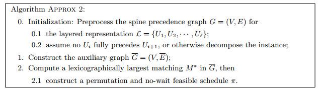
In the first step of the approximation algorithm Approx 2 (of which a high-level description is depicted in Fig. 4), an auxiliary undirected graph
Fig.3
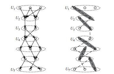
Fig.3
A spine precedence graph
A matching in
Lemma 7A lexicographically largest matching is a maximum matching in the graph
Proof By contradiction, we assume
Lemma 8A lexicographically largest matching in the graph
Proof Given an edge
Lemma 9A lexicographically largest matching
Proof Recall that we are constructing a permutation and no-wait schedule. Using the layer representation
Since the time-span for processing the jobs of the layer
This finishes the proof of the lemma.
The above analysis motivates the second step of the algorithm Approx 2, which is to compute a lexicographically largest matching
Fig.4
We have showed the makespan of the schedule achieved by the algorithm Approx 2 in Eq. (4). For the approximation ratio, we will prove next an improved lower bound on the minimum makespan using the matching
Recall that there are no adjacent
Lemma 10Let
Proof From
Let
Lemma 11.In the optimal schedule
Proof We assume to the contrary that the last machine idles for
To prove the claim, first from
Recall the important fact about a spine graph is that every job of
On the other hand, let
Let
This proves the lemma that the last machine idles for at least
Theorem 3The lexicographically largest matching based algorithm Approx 2 is an
Proof Recall that in the second step of the algorithm Approx 2, a lexicographically largest matching
By Lemma 11 and the fact that the defined time intervals
Using these lower bounds in Eqs. (1) and (5), we have
That is, Approx 2 is a
To prove the tightness of the ratio
Fig.5
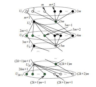
Fig.5
The spine precedence graph
when
4 Concluding remarks
We studied the precedence constrained scheduling of unit jobs on an open-shop and a flow-shop, in which the number
参考文献
Bounds for certain multiprocessing anomalies
[J].DOI:10.1002/j.1538-7305.1966.tb01709.x [本文引用: 3]
Optimization and approximation in deterministic sequencing and scheduling: A survey
[J].
Worst case analysis of two scheduling algorithms
[J].
A new insight into the Coffman-Graham algorithm
[J].DOI:10.1137/S0097539790181889 [本文引用: 2]
Precedence constrained scheduling in
DOI:10.1016/j.jcss.2008.04.001 [本文引用: 2]
Polynomial time approximation algorithms for machine scheduling: Ten open problems
[J].
A survey on how the structure of precedence constraints may change the complexity class of scheduling problems
[J].DOI:10.1007/s10951-017-0519-z [本文引用: 1]
On some variants of the bandwidth minimization problem
[J].
Identical parallel machines vs. chains in scheduling complexity
[J].DOI:10.1016/S0377-2217(02)00767-1 [本文引用: 6]
Open shop problems with unit time operations
[J].
Deterministic scheduling with pipelined processors
[J].
A polynomial algorithm for the
DOI:10.1016/0377-2217(94)90335-2 [本文引用: 2]
Complexity results for single-machine problems with positive finish-start time-lags
[J].DOI:10.1007/s006070050036 [本文引用: 2]
Open-shop scheduling for unit jobs under precedence constraints
[J].DOI:10.1016/j.tcs.2019.09.046 [本文引用: 6]
An
O nakhozhdenii maksimal'nogo potoka v setyakh spetsial'nogo vida i nekotorykh prilozheniyakh (in Russian; title translation: On finding maximum flows in networks with special structure and some applications)
[J].
Permutation vs. non-permutation flow shop schedules
[J].DOI:10.1016/0167-6377(91)90014-G [本文引用: 1]
